Overview
Five overarching sectors are developed to represent the broader energy system. Each of these includes a large set of technologies to capture the status of the current energy mix, as well as future technology options for decarbonisation. Specifically, the following sectors are modelled:
Primary energy supply – this relates to fossil fuel supply, nuclear fuel supply, renewable energy potential and hydrogen imports. Primary energy supply and transformation infrastructure (e.g., gas pipelines, LNG regasification terminals, oil refineries, etc.) is not modelled explicitly, with the only exception of electricity interconnectors between countries in the disaggregated version of the CLEWs-EU model and hydrogen production. Supply of biomass into the energy system occurs via an interlinkage with the land module of the model.
Electricity and heat generation – fossil fuel, nuclear and renewable energy technologies are represented, along with a simplified representation of grid networks to capture associated losses. Additional technology options represented include electricity storage, use of Carbon Capture and Storage (CCS) technologies, hydrogen production through electrolysers to produce green hydrogen and steam methane reforming (i.e., using natural gas as feedstock) with or without CCS to produce blue and grey hydrogen respectively.
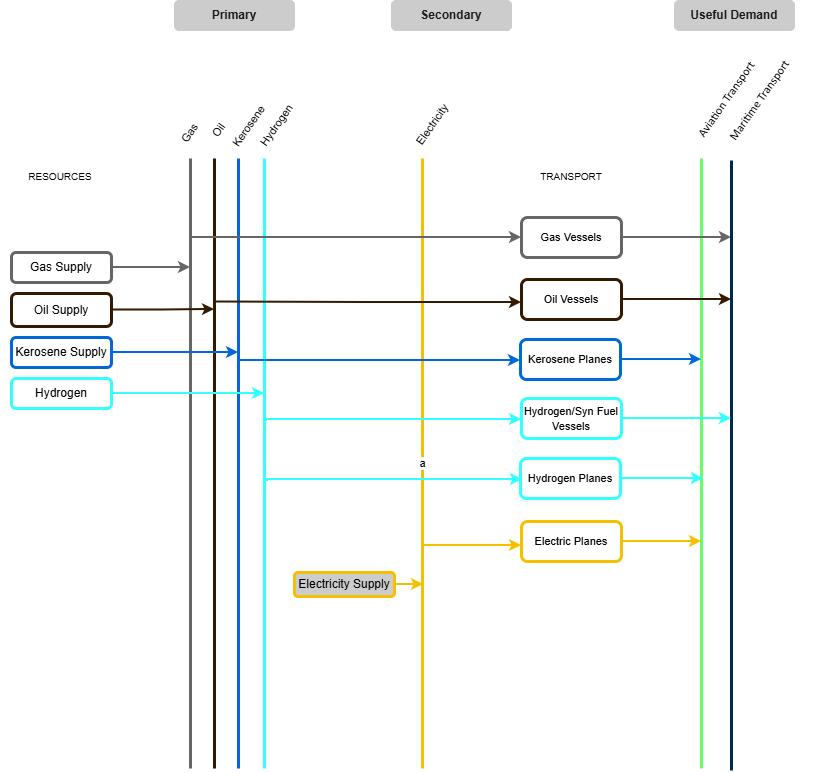
Transport – the transport sector includes road transport, which is further broken down to passenger (passenger cars and buses) and freight (light commercial vans and heavy trucks), rail transport (passenger and freight), aviation and shipping.
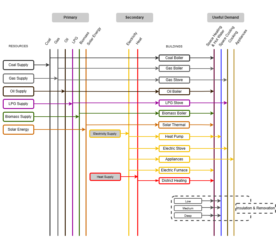
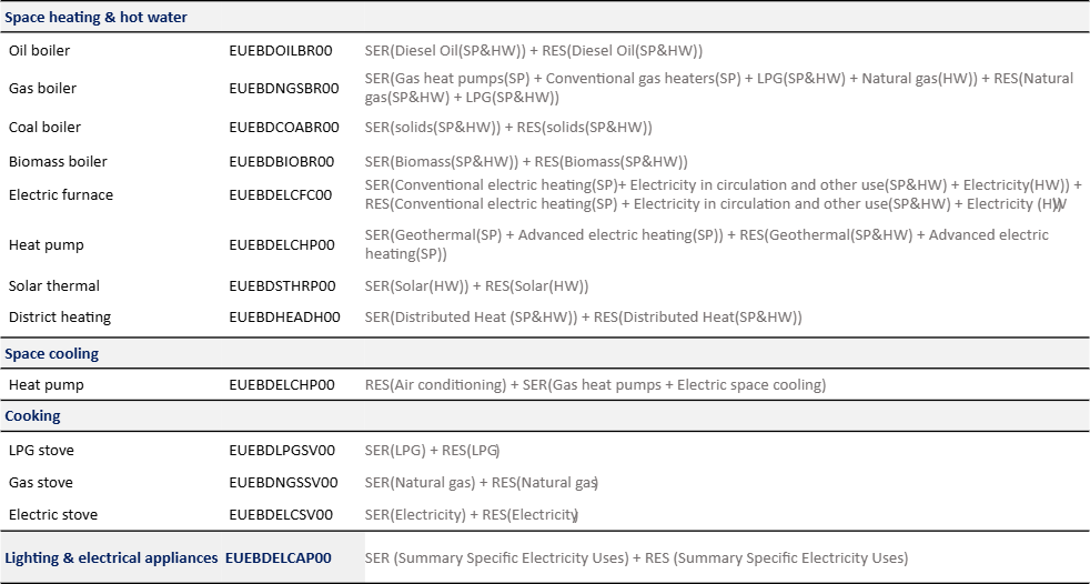
Buildings – this sector basically comprises of the households and service sectors. It is broken down into end-use services (i.e., space heating, space cooling, cooking, sanitary hot water, lighting and appliances).
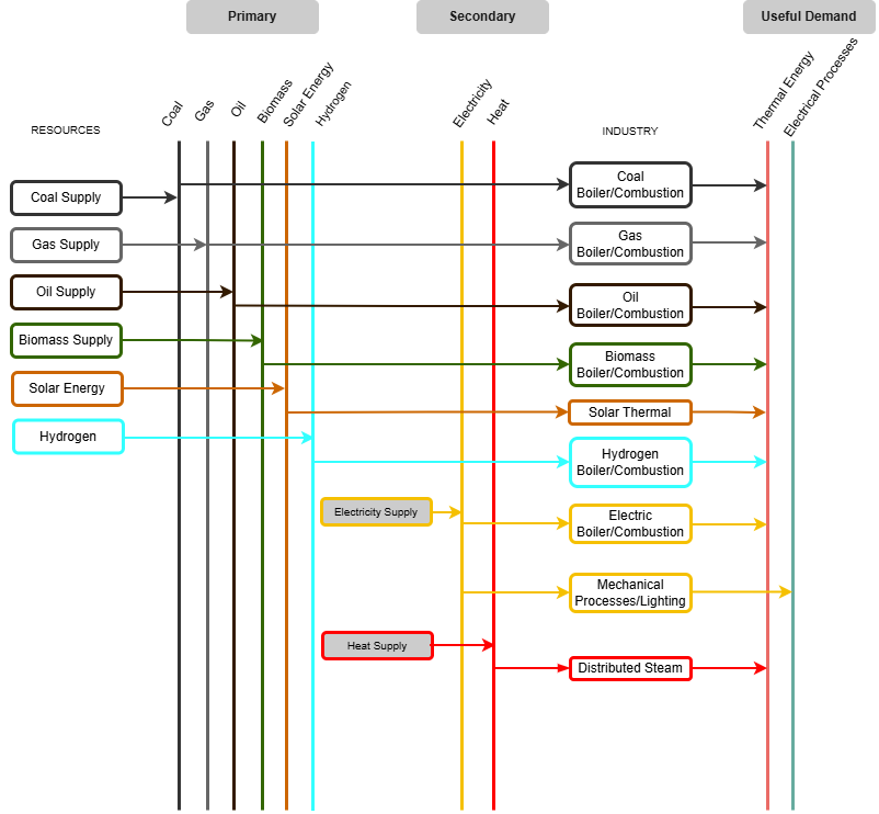
Industry –up to four distinct industries, based on the most energy-consuming sectors, are represented separately for each country, while the rest of the industries are lumped together in a fifth category . The output of each of the industries is represented in generic energy terms (i.e., PJ of useful energy services).
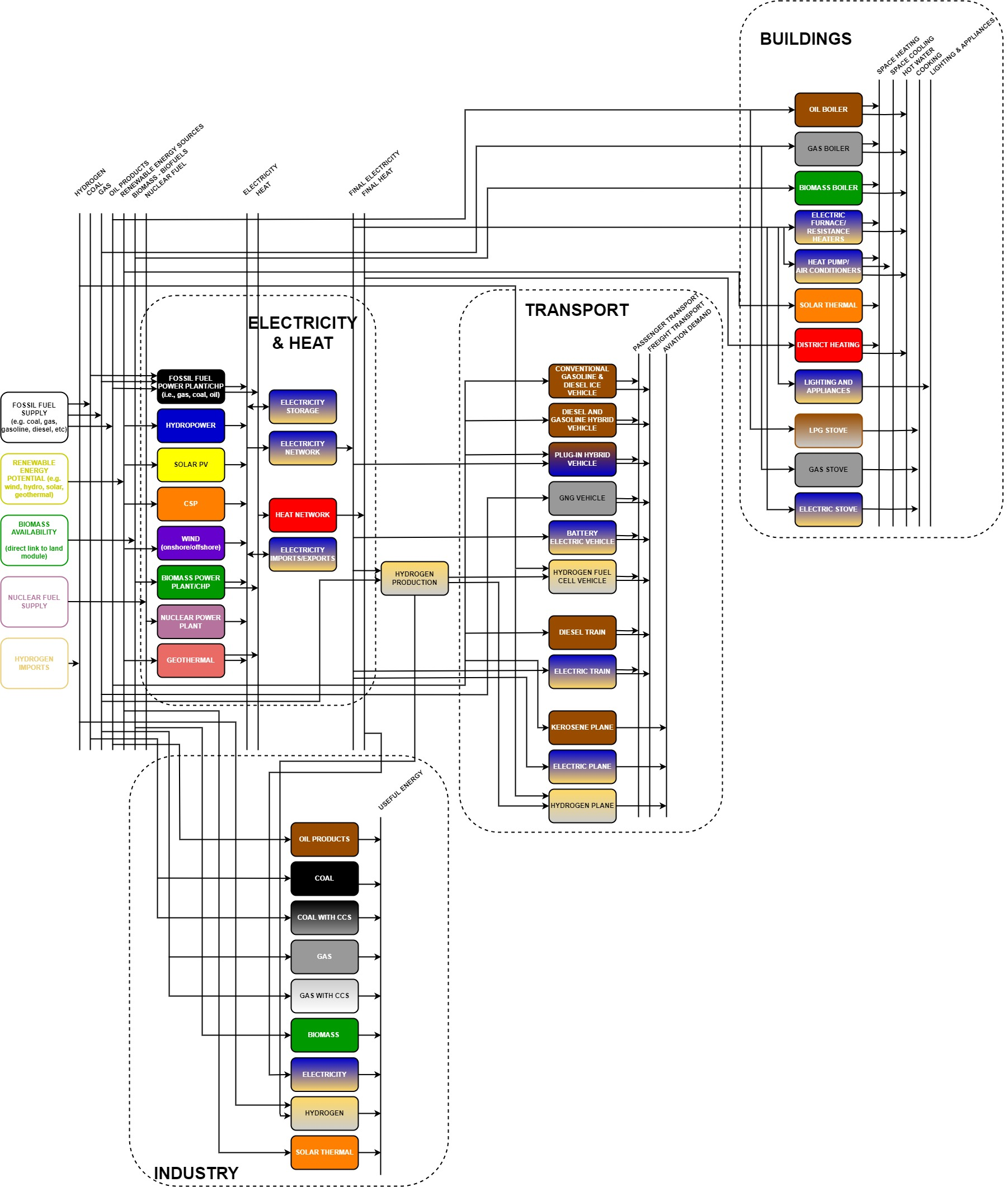
It should be noted that the energy demands in all sectors are inputs to the model . A simplified representation of the structure of the energy module is provided in Figure 2. Further disaggregation of technologies is available in the model than is depicted. For instance, the various vehicle technologies will be further broken down into passenger cars, buses, light commercial vans and heavy trucks. Similarly, the structure of the industrial sector will be constructed for each of the four key industries (and other industries) to be represented in each country.
Overarching assumptions
Among the most crucial assumptions adopted in the model are the international fuel price projections. The model uses as a base the international fuel price projections of the European Commission recommendations (European Commission – DG CLIMA, 2024). The same source provides projections on the existing Emission Trading System (ETS) and the new ETS (Table 1).
The existing ETS initially applied only to electricity and heat generation and energy-intensive industries. The new Emission Trading System (ETS2) will be expanded to include buildings, road transport, and smaller industries (i.e., those not already covered by the existing ETS), becoming fully operational in 2027 (European Commission – Directorate-General for Energy, n.d.-a). Both the ETS and the ETS2 are included in the baseline setup of the CLEWs-EU model.
Fuel / ETS |
Unit |
2021 |
2025 |
2030 |
2035 |
2040 |
2045 |
2050 |
|---|---|---|---|---|---|---|---|---|
Oil |
EUR2018/GJ |
10.24 |
10.16 |
11.39 |
12.62 |
12.95 |
14.10 |
16.14 |
Gas (NCV) |
EUR2018/GJ |
14.83 |
7.70 |
7.38 |
6.72 |
8.28 |
8.11 |
7.87 |
Coal |
EUR2018/GJ |
3.69 |
3.36 |
3.28 |
3.11 |
3.11 |
3.28 |
3.28 |
ETS WEM |
EUR2018/tCO₂ |
53.27 |
77.85 |
77.85 |
81.95 |
81.95 |
131.12 |
155.71 |
ETS WAM |
EUR2018/tCO₂ |
53.27 |
77.85 |
77.85 |
114.73 |
237.66 |
352.39 |
401.56 |
ETS2 WEM |
EUR2018/tCO₂ |
0 |
0 |
0 |
0 |
0 |
0 |
0 |
ETS2 WAM |
EUR2018/tCO₂ |
0 |
0 |
45.07 |
114.73 |
237.66 |
352.39 |
401.56 |
Electricity and heat generation
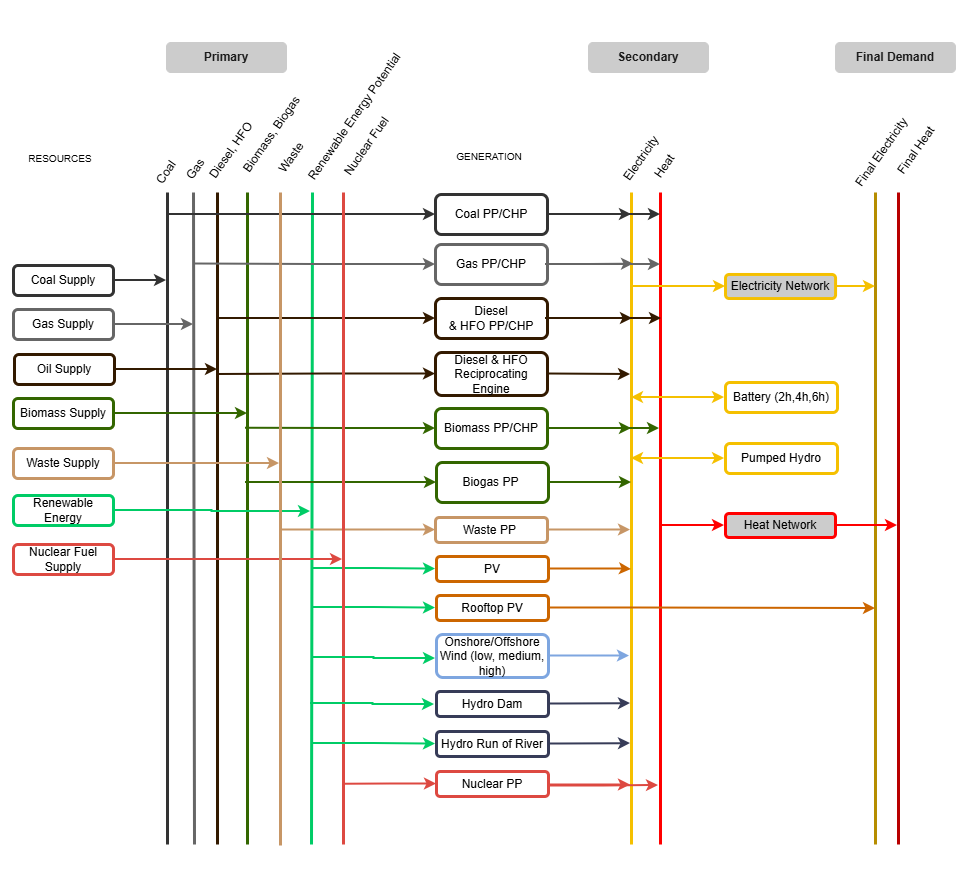
Representation of electricity and heat generation is crucial in the CLEWs-EU model as it defines the long-term cost-competitiveness of these commodities as alternatives to fuel combustion at the final consumer level. A large set of technologies is used to represent this sector (Figure 3). The following subsections discuss the structure and key assumptions adopted in this sector.
Electricity
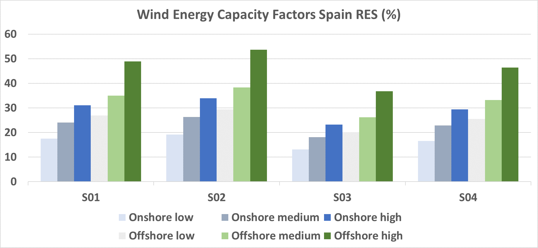
The development of the electricity supply module has been based on detailed historical data for electricity demand, PV and wind profiles, as well as hydro availability. Data on existing installed capacity has been retrieved primarily from the JRC-IDEES 2021 database (Rózsai et al., 2024) and cross-verified with data from ENTSO-E. Furthermore, demand profiles have been downloaded from the ENTSO-E website for the year 2022 for all member countries (ENTSO‑E, . Moreover, an important constraint is set, related to the maximum total installed capacity of RES power plants: for hydropower, these values are adopted from each country’s NECP projections, whereas for solar and wind energy, from the JRC ENSPRESO database (Ruiz et al., 2019). PV and wind generation profiles have been downloaded from Renewables-Ninja (Pfenninger & Staffell, 2022) and adjusted to get the average annual capacity factor based on Eurostat (Eurostat, 2025b). Wind and PV resources have been broken into high, average and low potential, based on data from the JRC-IDEES database (Rózsai et al., 2024) (Figure 4). For each country, there are 3 PV and wind technologies/resources associated with a different capacity factor (%) and economic potential (in GW).
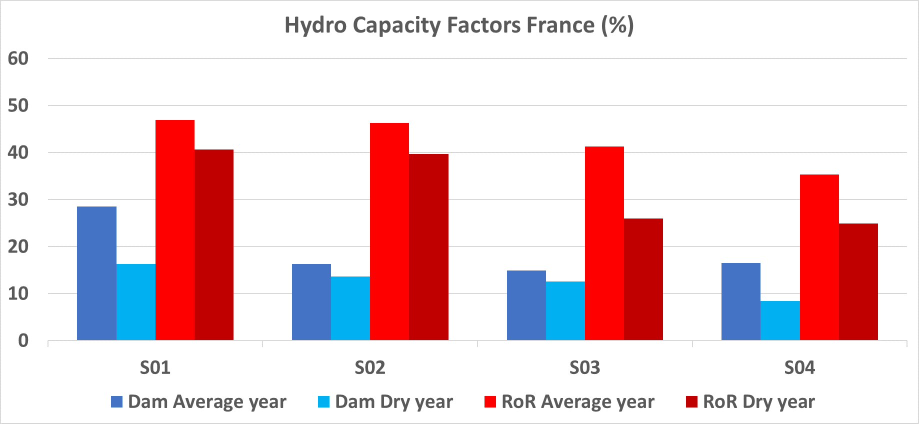
Run-of-River (RoR) hydro generation is modelled similarly as in the case of PV and wind, using a historical profile of generation, retrieved from ENTSO-E (ENTSO‑E, 2025) and adjusted to get the average capacity factor based on historical data by Eurostat (Eurostat, 2025b). The hourly profiles of demand, as well as generation from PV, wind and RoR have been treated and adjusted to the agreed temporal resolution that is used across the CLEWs-EU model (see Section 1.2.3). Hydro plants with dams are modelled as generators running on water (represented as a “fuel”), while the maximum capacity factor is capped based on historical generation. The main difference between RoR and hydro with dams is that hydro with dams can operate flexibly, subject to a seasonal cap on generation that is based on statistical analysis of historical hydro generation data for seven consecutive years. To better reflect the annual fluctuations of hydropower generation, the model considers 7-year cycles where 6 years with average hydrological data are followed by a single ”dry” year (Figure 5). All adopted profiles for hydro, PV, and wind have been compared with historical data based on Eurostat and have been treated to represent an average year. For this purpose, historical annual averages have been obtained from 1980-2019 for PV and Wind and 2015-2022 for hydro.
The model accounts for a wide range of technologies which comprise a portfolio of projects to be considered in the optimisation. The technological mix of conventional generators can be distinguished based on the thermodynamic cycle (steam (ST) vs gas, open vs closed cycle vs combined cycle (CCGT)), and on the fuel (biomass, nuclear, coal, natural gas, liquid fuels, waste, biogas etc.). The model also includes CCS for specific technologies, coal-ST with CCS, gas CCGT with CCS and biomass-ST with CCS. Utilising data from ENTSO-E (ENTSO‑E, , grid interconnections between the EU member states are represented in the model. Specifically, the existing and potential future capacities of interconnections have been incorporated in the model. The level of electricity trade between the systems is endogenously calculated in the model and it depends on the technoeconomic assumptions adopted for each scenario. The techno-economic parameters of electricity generation technologies (efficiency, capital cost, operation and maintenance cost, etc.), presented in Table 2 and Table 3, are based on the latest available EU Reference Scenario (European Commission - Directorate General for Energy. et al., 2021). The CLEWS-EU model considers two types of electricity storage, namely battery energy storage systems (BESS) and pumped hydro. The techno-economic parameters and trajectories for these storage options have been based on the Annual Technology Baseline (ATB) documentation of NREL (NREL, 2024). The model assumptions include capital cost trajectories for all technologies; this is especially important for technologies where the capital cost is expected to be reduced with time as in the case of PV, wind and BESS. The OSeMOSYS code used to run the CLEWs-EU model contains modified storage equations to ensure proper representation of the operation of these technologies.
Technology |
CAPEX 2021 |
CAPEX 2030 |
CAPEX 2050 |
FOM 2021 |
FOM 2030 |
FOM 2050 |
|---|---|---|---|---|---|---|
Nuclear Generation III |
4,770 |
4,500 |
4,500 |
120 |
115 |
105 |
Coal supercritical |
1,650 |
1,650 |
1,650 |
33–41 |
31–36 |
28–31 |
Coal Supercritical with CCS |
3,432 |
3,270 |
3,075 |
69 |
66 |
62 |
Biomass Steam Turbine |
1,980 |
1,800 |
1,700 |
47 |
40 |
38 |
Biomass Steam Turbine with CCS |
4,013 |
3,675 |
3,205 |
80 |
69 |
61 |
Steam Turbine CHP |
1,980 |
1,800 |
1,700 |
46 |
40 |
38 |
Gas Turbine CC |
598 |
579 |
570 |
22 |
21 |
19 |
Gas Turbine OC * |
399–497 |
386–465 |
380–450 |
12–29 |
12–24 |
12–24 |
Reciprocating engine |
1,897 |
1,897 |
1,897 |
35 |
35 |
35 |
Natural Gas CC with CCS |
1,738 |
1,625 |
1,500 |
41 |
38 |
34 |
Geothermal |
3,211 |
2,807 |
2,614 |
102 |
95 |
99 |
Waste PP |
1,647 |
1,615 |
1,600 |
52 |
45 |
39 |
Hydro reservoir PP |
2,100 |
2,100 |
2,100 |
26 |
26 |
26 |
Run of river PP |
1,711 |
1,670 |
1,650 |
9 |
8 |
8 |
Batteries ** |
578–1734 |
380–1140 |
300–900 |
48 |
31 |
21 |
Pumped Hydro Storage |
3,062 |
30,612 |
3,062 |
19 |
19 |
19 |
Technology |
CAPEX 2021 |
CAPEX 2030 |
CAPEX 2050 |
FOM 2021 |
FOM 2030 |
FOM 2050 |
|---|---|---|---|---|---|---|
Wind onshore Low |
1198 |
1175 |
1100 |
13 |
13 |
12 |
Wind onshore Medium |
1045 |
1000 |
925 |
14 |
14 |
12 |
Wind onshore High |
995 |
950 |
880 |
21.9 |
21 |
20 |
Wind offshore Low |
1778 |
1650 |
1503 |
32.4 |
27 |
26 |
Wind offshore Medium |
1756 |
1622 |
1468 |
32.4 |
27 |
26 |
Wind offshore High |
1734 |
1593 |
1432 |
32.4 |
27 |
26 |
Solar PV Low |
470 |
400 |
367 |
14.8 |
12.6 |
8.2 |
Solar PV Medium |
455 |
387 |
355 |
14.8 |
12.6 |
8.2 |
Solar PV High |
447 |
380 |
348 |
14.8 |
12.6 |
8.2 |
Solar PV Rooftop Low |
470 |
400 |
367 |
18.6 |
14.9 |
9 |
Solar PV Rooftop Medium |
635 |
543 |
500 |
18.6 |
14.9 |
9 |
Solar PV Rooftop High |
625 |
536 |
493 |
18.6 |
14.9 |
9 |
Heat
The heat module of the power sector of the CLEWs-EU model contains CHP plants with the main purpose of producing electricity, while heat is directed as a by-product into district heating networks. The existing capacity of CHP plants and the level of district heating demand are retrieved from the JRC-IDEES 2021 database (Rózsai et al., 2024). CHP units that are part of industrial facilities are excluded from this module, as end-use energy demand in the industry sector is accounted for separately. To vary the level of electricity and heat production throughout the model horizon and the intra-annual timesteps, we have added two modes of operation for each CHP technology. The first mode represents the maximum rate of electricity production for the CHP unit, while the highest heat-rate production is accounted for in the other mode. The electricity and heat efficiency ranges of CHPs for these two modes are taken from IEA ETSAP (IEA ETSAP, 2010). Depending on the level of electricity versus heat demand in the end-use sectors, the model chooses which of the two modes to prioritise.
Units of electricity and heat generation technologies
OSeMOSYS models do not have a specific unit definition, so the decision on the units to be used is entirely up to the modeller. The parameter “CapacityToActivityUnit” is used to relate the rate of activity of each technology to its capacity. In the energy module of CLEWs-EU, this parameter is either 1 or 31.536. In the former case, this means that the activity is in PJ and the capacity is in PJ/year, while in the latter case, the capacity is in GW.
Capacity |
Activity |
Capital cost |
Fixed cost |
Variable cost |
|---|---|---|---|---|
GW |
PJ |
Million EUR2018/GW |
Million EUR2018/GW |
Million EUR2018/PJ |
Buildings
The buildings module aggregates the residential and commercial services sectors. It splits demand for energy services into four primary end-uses: heating (i.e., space heating & hot water), space cooling, cooking and electrical appliances. Units for the capacity and cost characteristics of electricity and heat technologies in the CLEWs-EU model. For space heating, the module incorporates several technologies to reflect the heterogeneity of heating systems in buildings. These include solid fuel furnaces for solid fuels, oil boilers for LPG and gas/diesel oil, gas-based systems (including gas heat pumps and heaters), biomass boilers for biomass and waste, district heating systems, heat pumps (indicated as advanced electric heating in JRC-IDEES database (Rózsai et al., 2024)), electric furnaces (representing conventional electric heating and circulation systems), and solar thermal installations. Space cooling is represented by electric space cooling systems due to the predominance of electricity-based cooling technologies in both residential and commercial buildings. Cooking is represented using three primary technologies: LPG stoves, gas stoves, and electric stoves, capturing the most common cooking appliances across the sectors. Lighting and electrical appliances are treated as a single, aggregated category without further technological disaggregation. As in all modules of CLEWs-EU, to facilitate the independent development and testing of the buildings’ module, we introduce additional dummy technologies for electricity and centralised heat provision, as well as dummy technologies that can directly satisfy the defined energy service demands at an exceptionally high cost. These temporary additions allow for standalone operation of the module during development phases. However, it’s important to note that these dummy technologies are also included in the final integrated model version, where electricity and heat are endogenous to the model via the dedicated “Electricity & Heat generation” module, as they allow identification of potential modelling faults.
Technoeconomic characteristics of building technology options
The development of the buildings module was based on data from the Joint Research Centre of the European Commission, specifically the Joint Research Centre’s Integrated Database of the European Energy System (JRC-IDEES). The latest version of the publicly-available dataset, JRC-IDEES-2021 (Rózsai et al., 2024) was published in May 2024 and covers the timeframe from 2000 to 2021, making it suitable for the calibration of the model. The release introduces several methodological refinements and incorporates new statistical sources as well as feedback from the user community. As an analytical database, it goes beyond raw statistical data by processing and decomposing energy consumption into specific processes and end-uses, allowing for in-depth analysis of energy system dynamics. JRC-IDEES was created by harmonizing existing statistics with technical assumptions. For the buildings sector (both commercial and residential), JRC-IDEES (Rózsai et al., 2024) offers highly disaggregated data on energy demand, breaking it down by end-use (e.g., space heating, cooling, lighting) and fuel type and is aligned with Eurostat energy balances. As per the overarching model assumptions (Table 5), capital costs are derived from the EU Reference Scenario 2020 technology assumptions (European Commission - Directorate General for Energy. et al., 2021), with the exception of solid fuel boilers/furnaces, which are taken from IEA ETSAP (IEA ETSAP, 2012), which is also consulted to derive operation and maintenance costs.
Technology |
Capital cost (EUR2018/kW) |
Fixed O&M (EUR2018/kW) |
Energy Intensity Index (2021 = 100%) |
||||||
|---|---|---|---|---|---|---|---|---|---|
2021 |
2030 |
2050 |
2021 |
2030 |
2050 |
2021 |
2030 |
2050 |
|
Oil boiler |
170 |
192 |
180 |
5.08 |
5.08 |
5.08 |
100% |
100% |
100% |
Gas boiler |
165 |
187 |
185 |
5.08 |
5.08 |
5.08 |
100% |
88% |
88% |
Coal boiler |
165 |
187 |
185 |
5.08 |
5.08 |
5.08 |
100% |
100% |
100% |
Biomass boiler |
431 |
488 |
457 |
13.22 |
13.22 |
13.22 |
100% |
94% |
91% |
Electric furnace |
64 |
78 |
71 |
5.08 |
5.08 |
5.08 |
100% |
100% |
100% |
Heat pump |
817 |
865 |
697 |
5.08 |
5.08 |
5.08 |
100% |
81% |
63% |
Solar thermal |
1308 |
1432 |
1119 |
5.08 |
5.08 |
5.08 |
100% |
95% |
92% |
District heating |
96 |
111 |
104 |
— |
— |
— |
100% |
99% |
99% |
Heat pump (cooling) |
817 |
865 |
697 |
5.08 |
5.08 |
5.08 |
100% |
81% |
66% |
LPG stove |
198 |
202 |
195 |
— |
— |
— |
100% |
95% |
91% |
Gas stove |
198 |
202 |
195 |
— |
— |
— |
100% |
95% |
91% |
Electric stove |
189 |
194 |
186 |
— |
— |
— |
100% |
96% |
91% |
General appliances |
— |
— |
— |
— |
— |
— |
100% |
93% |
91% |
Renovation (Low) |
1134 |
1134 |
1134 |
— |
— |
— |
100% |
100% |
100% |
Renovation (Medium) |
705 |
705 |
705 |
— |
— |
— |
100% |
100% |
100% |
Renovation (High) |
900 |
900 |
900 |
— |
— |
— |
100% |
100% |
100% |
Efficiency factors are projected to evolve and are therefore inserted in the model as time series. For the period 2018-2021, these calculations were based on the JRC-IDEES-2021 database. Since both Final Energy Consumption (FEC) and Useful Energy Consumption (UEC) data for the Households (HH) and Services (SER) sectors are available in the database for all EU Member States and the European Union as a whole, we computed the efficiency factors as:
Efficiency = \(\frac{\text{Total UEC}}{\text{Total FEC}}\)
For 2022-2050 projections, efficiencies are indexed to the estimated efficiencies for 2021 from JRC-IDEES as:
Efficiency \((y_n) = Efficiency_{2021} \times Energy\ Intensity\ Index\)
Where
\(Energy\ Intensity\ Index = \frac{Efficiency\ in\ Reference\ Scenario\ (y_n)}{Efficiency\ in\ Reference\ Scenario_{2021}}\),
derived from the EU Reference Scenario 2020 technology assumptions.
Some technologies, such as oil- and coal-based systems, are assumed to maintain constant efficiency over time. For lighting and electrical appliances, the model incorporates projected efficiency improvements due to equipment replacement and anticipated technological advancements. This is implemented by gradually improving the relevant efficiency parameters over time, reflecting the expected enhancement in energy conversion efficiency for these end-uses.
Furthermore, according to the adopted technoeconomic assumptions, building renovation costs and savings potential are assumed to differ across EU regions, since both climatic and socioeconomic conditions influence renovation performance. EU Member States are grouped as follows:
South: Greece, Cyprus, Italy, Spain, Malta, Portugal
East: Bulgaria, Estonia, Latvia, Lithuania, Romania
Centre/West: Austria, Belgium, Czech Republic, Germany, France, Croatia, Hungary, Ireland, Luxembourg, Netherlands, Poland, Slovenia, Slovakia
North: Denmark, Finland, Sweden
A limitation on annual renovation rates is also implemented in the model. Specifically, up to \(1.5\%\) of the building stock may be renovated per year, unless adjusted in a scenario.
Region |
Extent of renovation |
Energy savings (%) |
Capital cost (Million EUR2018/PJ annual savings) |
|---|---|---|---|
Centre/West |
Light renovation |
15.8% |
1134 |
Centre/West |
Medium renovation |
68.7% |
705 |
Centre/West |
Deep renovation |
78.0% |
900 |
North |
Light renovation |
22.3% |
897 |
North |
Medium renovation |
67.4% |
749 |
North |
Deep renovation |
86.6% |
870 |
South |
Light renovation |
16.1% |
853 |
South |
Medium renovation |
56.5% |
682 |
South |
Deep renovation |
75.3% |
802 |
East |
Light renovation |
12.9% |
780 |
East |
Medium renovation |
55.5% |
452 |
East |
Deep renovation |
68.6% |
566 |
Finally, technology lifetimes are also sourced from available technology briefs (IEA ETSAP, 2012), which provide standardised estimates for the operational lifespan of various heating and cooling technologies in residential and commercial buildings.
Input data transformation
Due to the lower technological complexity adopted in CLEWs-EU, aggregation from the relevant input data is pursued. Specifically, we group similar technologies together to keep the model complexity low and to create meaningful categories for analysis. Energy service demands for the tertiary and residential sectors are aggregated together. JRC-IDEES (Rózsai et al., 2024) provided data for the use of hot water separately, but we group this thermal demand with space heating.
Building demand projections
Demand projections in the baseline scenario of CLEWs-EU are based on final energy demand projections for the residential and commercial sectors, retrieved from the EU Reference Scenario 2020 (European Commission - Directorate General for Energy. et al., 2021). For consistency with the JRC-IDEES-2021 data used for the calibration of the model, we indexed the values of the final energy demand projections to the base year 2021 and calculated coefficients relative to this baseline. Specifically, in the baseline setup of the CLEWs-EU model, the growth rate of useful energy demand for each of the energy service demands in the period 2022-2050 resembles the collective final energy demand growth rate of the residential and tertiary sectors from the EU Reference Scenario 2020 (European Commission - Directorate General for Energy. et al., 2021). This implies that the overall efficiency will remain at current levels until mid-century. However, since the model allows building upgrades for improved energy efficiency, as well as assumes partial improvement of the energy efficiency of the technology stock for the various energy services, the baseline scenario of CLEWs-EU is expected to result to lower final energy demand projections than the EU Reference Scenario 2020. This is an aspect that can be adjusted in the scenario exploration phase of the DIAMOND project (i.e., WP5). More details on the exact demand projections by country and energy service are provided in the Supplementary material within the model’s GitHub repository.
Units of building sector technologies and commodities
Since OSeMOSYS models do not have a specific unit definition, the adopted units must be defined externally prior to the model development. As indicated in the tables below, the output of building technologies is defined in terms of their activity. The existing capacity of technologies is estimated based on the activity of technologies as extracted from the JRC-IDEES 2021 database.
Energy service technologies |
Input |
Output |
|---|---|---|
Space heating & hot water |
PJ fuel |
PJ of useful energy for heating |
Space cooling |
PJ electricity |
PJ of useful energy for cooling |
Cooking |
PJ fuel |
PJ of useful thermal energy for cooking |
Appliances |
PJ electricity |
PJ of useful energy for appliances |
Energy efficiency upgrades |
— |
PJ of useful energy savings (cooling & heating) |
Technology |
Capacity |
Capital cost |
Fixed cost |
|---|---|---|---|
Space heating & hot water |
GW |
Million EUR2018/GW |
Million EUR2018/GW |
Space cooling |
GW |
Million EUR2018/GW |
Million EUR2018/GW |
Cooking |
GW |
Million EUR2018/GW |
Million EUR2018/GW |
Appliances |
PJ/year |
— |
— |
Energy efficiency upgrades |
PJ/year |
Million EUR2018/PJ yearly savings |
— |
Industry
Representation of industry in the CLEWs-EU model is largely based on data retrieved from the JRC-IDEES 2021 database (Rózsai et al., 2024). Specifically, the database provides statistics on the final energy demand and useful energy demand for each sector by process and by technology/fuel for the period 2000-2021, but for the purposes of CLEWs-EU, we only focused on the period 2018-2021.
As a first step, the key industrial sectors in each country are identified based on the level of final energy demand in 2021 (Table 2); for each country, up to 4 main sectors are represented separately, while the rest of the sectors are aggregated into an “Other industrial sectors” category. In countries where industrial energy demand is low, the number of sectors represented is lower (e.g., Cyprus, Luxembourg, Malta, etc.). As mentioned above, the output of each of the industries is represented in generic energy terms (i.e., PJ of useful energy services). As more data becomes available in the future after completion of the DIAMOND project, a more explicit representation of key industries can be pursued.
Country |
ISI |
NFM |
CHI |
NMM |
PPA |
FBT |
TRE |
MAE |
TEL |
WWP |
OIS |
|---|---|---|---|---|---|---|---|---|---|---|---|
AT |
X |
X |
X |
X |
|||||||
BE |
X |
X |
X |
X |
X |
||||||
BG |
X |
X |
X |
X |
X |
||||||
CY |
X |
X |
X |
||||||||
CZ |
X |
X |
X |
X |
|||||||
DE |
X |
X |
X |
X |
|||||||
DK |
X |
X |
X |
X |
X |
||||||
EE |
X |
X |
X |
X |
X |
||||||
GR |
X |
X |
X |
X |
X |
||||||
ES |
X |
X |
X |
X |
|||||||
FI |
X |
X |
X |
X |
|||||||
FR |
X |
X |
X |
X |
X |
||||||
HR |
X |
X |
X |
X |
X |
||||||
HU |
X |
X |
X |
X |
X |
||||||
IE |
X |
X |
X |
X |
X |
||||||
IT |
X |
X |
X |
X |
|||||||
LT |
X |
X |
X |
X |
X |
||||||
LU |
X |
X |
X |
||||||||
LV |
X |
X |
X |
X |
|||||||
MT |
X |
||||||||||
NL |
X |
X |
X |
X |
|||||||
PL |
X |
X |
X |
X |
|||||||
PT |
X |
X |
X |
X |
X |
||||||
RO |
X |
X |
X |
X |
X |
||||||
SE |
X |
X |
X |
X |
|||||||
SI |
X |
X |
X |
X |
|||||||
SK |
X |
X |
X |
X |
Technoeconomic characteristics of industrial technology options
Data on final energy demand and useful energy demand are aggregated for each fuel category in each of the represented sectors, and an efficiency is calculated for the years 2018–2021. Specifically, the technological and fuel options for satisfying useful energy demand are the following:
Thermal energy – coal (with and without CCS), oil, natural gas (with and without CCS), biomass/biofuels, hydrogen, solar thermal, centralised steam, electricity.
Electrical processes (lighting, motor drives, etc.) – electricity.
Adopting the same approach as for the buildings sector, projections for the evolution of capital costs and efficiencies of industrial boilers until 2050 are based on assumptions from the EU Reference Scenario 2020 (European Commission - Directorate General for Energy et al., 2021). However, efficiency is indexed to the last available year of statistics (i.e. 2021), using data from the JRC-IDEES 2021 database (Rózsai et al., 2024).
An overview of the key technoeconomic assumptions for the industrial sector is provided in Table 11.
Technology |
Capital cost (EUR2018/kW) |
Fixed O&M (EUR2018/kW) |
Energy Consumption Index (2021=100%) |
||||||
|---|---|---|---|---|---|---|---|---|---|
2021 |
2030 |
2050 |
2021 |
2030 |
2050 |
2021 |
2030 |
2050 |
|
Oil |
232 |
252 |
252 |
1.32 |
1.32 |
1.32 |
100% |
91% |
91% |
Coal |
356 |
386 |
386 |
1.37 |
1.37 |
1.37 |
100% |
91% |
91% |
Coal with CCS* |
2203 |
2085 |
1888 |
38.37 |
35.01 |
30.46 |
115% |
114% |
107% |
Gas |
119 |
128 |
128 |
1.25 |
1.25 |
1.25 |
100% |
92% |
92% |
Gas with CCS* |
1350 |
1256 |
1133 |
22.75 |
20.14 |
16.09 |
132% |
126% |
121% |
Biomass |
771 |
836 |
836 |
1.37 |
1.37 |
1.37 |
100% |
92% |
92% |
Electricity (heat) |
701 |
683 |
673 |
10.36 |
10.36 |
10.36 |
100% |
100% |
100% |
Electrical processes |
— |
— |
— |
— |
— |
— |
100% |
94% |
87% |
Hydrogen |
119 |
128 |
128 |
1.25 |
1.25 |
1.25 |
100% |
92% |
92% |
Solar thermal |
1308 |
1432 |
1119 |
15.54 |
15.54 |
15.54 |
100% |
95% |
92% |
Data extraction and preparation from JRC-IDEES statistics to data ready for direct input to the model has been conducted with specially developed Python scripts. These scripts provide detail on the technology/fuel aggregation for each industry and how the selected industries vary across the countries and are made available on the model’s GitHub repository.
Industrial demand projections
In the baseline setup of the model, the growth rate of useful energy demand for the period 2022-2050 resembles the final energy demand growth rate of energy-intensive and non-energy intensive industries from the EU Reference Scenario 2020. Energy intensive industries include iron and steel, non-ferrous metals, chemicals, non-metallic minerals and pulp and paper; these are assumed to be subject to the existing Emissions Trading System (ETS). The rest of the industrial sectors are assumed to be subject to the new ETS (i.e., ETS2) from 2027 onwards (European Commission - Directorate-General for Energy, n.d.-a). Adopting the same growth rate for useful demand as for final energy demand from the EU Reference Scenario 2020 entails the assumption that the overall efficiency will remain at current levels until mid-century; this is an aspect that can be amended in the scenario exploration phase of the DIAMOND project (i.e., WP5). Separate demand projections are developed for each of the key industries of each member state. In turn, these are split between demand for useful thermal energy and useful demand for electrical processes; as indicated above, the latter is satisfied by a single technology option. More details on the exact demand projections by country and industrial sector are provided in the Supplementary material within the model’s GitHub repository.
Units of industrial sector technologies and commodities
OSeMOSYS models do not have a specific unit definition; as such, the adopted units must be defined externally before the model development. As indicated in the tables below, the output and capacity of industrial technologies are defined in terms of their activity. The existing capacity of technologies is estimated based on the activity of technologies as extracted from the JRC-IDEES 2021 database.
Technology |
Input |
Output |
Capacity |
Capital cost & Fixed cost |
Fuel cost |
|---|---|---|---|---|---|
Thermal & electrical processes |
PJ fuel |
PJ of useful heat |
GW |
Million EUR2018/GW |
Million EUR2018/PJ |
Transport
Similar to the other sectors of the energy system, the representation of the transport sector is constructed using data from the JRC-IDEES 2021 database (Rózsai et al., 2024). Specifically, relevant statistics are retrieved on the biofuel blending ratios in each mode of transport, existing stock of technologies, annual rate of activity and current efficiency levels of each technology. Key assumptions (e.g., efficiencies, annual mileage etc.) vary considerably between member states, hence country-specific information is adopted. Table 13 summarises the technology options represented for each mode of transport. As in the case of the industrial sector, Python scripts have been used for the transport data preparation and are also made available in the model’s GitHub repository.
Mode of transport |
Category |
Technology options |
|---|---|---|
Road transport |
Passenger cars |
Gasoline vehicles, Diesel vehicles, CNG/LNG vehicles, LPG vehicles, Hybrid electric vehicles, Plug-in electric vehicles, Battery electric vehicles, Hydrogen fuel cell vehicles |
Buses |
Diesel bus, CNG bus, Battery electric bus, Hydrogen fuel cell bus |
|
Light commercial vans |
Gasoline light trucks, Diesel light trucks, CNG/LNG light trucks, Hybrid electric light trucks, Plug-in electric light trucks, Battery electric light trucks, Hydrogen fuel cell light trucks |
|
Heavy trucks |
Diesel heavy trucks, CNG/LNG heavy trucks, Hybrid electric heavy trucks, Battery electric heavy trucks, Hydrogen fuel cell heavy trucks |
|
Rail transport |
Passenger |
Diesel train, Electric train |
Freight |
Diesel train, Electric train |
|
Aviation |
– |
Conventional kerosene planes, Electric planes, Hydrogen/e-fuel planes |
Shipping |
– |
Oil vessels, LNG vessels, Hydrogen/synthetic-fuel vessels |
Technoeconomic characteristics of mobility technology options
Technoeconomic characteristics of the various technologies and the evolution of the mobility demand for each mode of transport are based on the equivalent assumptions from the EU Reference Scenario 2020 (European Commission - Directorate General for Energy. et al., 2021), but are adjusted to agree with the base year statistics. Specifically, efficiency for each transport technology from JRC-IDEES in 2021 in each country is used as the starting point and its evolution is indexed to the growth rate projected in the EU Reference Scenario for the period up to 2050. In addition, the capital cost of transport technologies is based on the relevant technology assumptions of the EU Reference Scenario 2020, but the adopted number of technologies is lower for the sake of simplification. For instance, in the case of passenger vehicles, the corresponding values for medium cars are chosen for each technology option and these act as representative technologies.
Mode |
Technology |
Unit |
2021 |
2025 |
2030 |
2040 |
2050 |
|---|---|---|---|---|---|---|---|
Passenger road |
Gasoline vehicles |
EUR2018/vehicle |
20,084 |
20,140 |
20,794 |
21,553 |
23,431 |
Diesel vehicles |
EUR2018/vehicle |
23,540 |
23,685 |
24,366 |
25,833 |
34,858 |
|
CNG/LNG vehicles |
EUR2018/vehicle |
22,239 |
22,295 |
22,949 |
23,709 |
25,586 |
|
LPG vehicles |
EUR2018/vehicle |
21,652 |
21,708 |
22,361 |
23,121 |
24,998 |
|
Hybrid electric vehicles |
EUR2018/vehicle |
22,450 |
21,699 |
21,854 |
21,985 |
22,264 |
|
Plug-in electric vehicles |
EUR2018/vehicle |
26,673 |
23,419 |
22,296 |
21,967 |
21,973 |
|
Battery electric vehicles |
EUR2018/vehicle |
37,319 |
34,664 |
24,709 |
22,919 |
22,396 |
|
Hydrogen fuel cell vehicles |
EUR2018/vehicle |
49,782 |
37,348 |
31,330 |
29,985 |
30,170 |
|
Diesel bus |
EUR2018/vehicle |
287,109 |
287,844 |
290,033 |
291,898 |
294,695 |
|
CNG bus |
EUR2018/vehicle |
312,165 |
312,900 |
315,089 |
316,954 |
319,751 |
|
Electric bus |
EUR2018/vehicle |
444,300 |
420,053 |
329,131 |
308,306 |
299,329 |
|
Hydrogen fuel cell bus |
EUR2018/vehicle |
576,118 |
402,723 |
343,597 |
328,325 |
328,729 |
|
Freight road |
Gasoline light trucks |
EUR2018/vehicle |
18,535 |
18,608 |
19,880 |
22,328 |
27,952 |
Diesel light trucks |
EUR2018/vehicle |
23,336 |
23,571 |
25,683 |
31,935 |
31,935 |
|
CNG/LNG light trucks |
EUR2018/vehicle |
20,701 |
20,774 |
22,046 |
24,494 |
30,118 |
|
Hybrid electric light trucks |
EUR2018/vehicle |
25,316 |
24,340 |
24,479 |
24,651 |
24,872 |
|
Plug-in electric light trucks |
EUR2018/vehicle |
29,346 |
25,619 |
24,518 |
24,224 |
24,359 |
|
Battery electric light trucks |
EUR2018/vehicle |
37,489 |
35,018 |
25,755 |
22,940 |
22,117 |
|
Hydrogen fuel cell light trucks |
EUR2018/vehicle |
45,010 |
35,109 |
29,449 |
28,300 |
28,633 |
|
Diesel heavy trucks |
EUR2018/vehicle |
82,977 |
83,760 |
85,202 |
87,326 |
90,454 |
|
CNG/LNG heavy trucks |
EUR2018/vehicle |
102,438 |
103,221 |
104,663 |
106,787 |
109,914 |
|
Hybrid electric heavy trucks |
EUR2018/vehicle |
91,463 |
88,932 |
88,031 |
87,698 |
88,517 |
|
Battery electric heavy trucks |
EUR2018/vehicle |
182,915 |
170,477 |
123,834 |
107,803 |
103,601 |
|
Hydrogen fuel cell heavy trucks |
EUR2018/vehicle |
273,991 |
171,693 |
132,082 |
118,724 |
119,183 |
|
Passenger rail |
Diesel train |
MillionEUR2018/unit |
9.2 |
9.3 |
9.4 |
9.7 |
10.1 |
Electric train |
MillionEUR2018/unit |
12.6 |
12.7 |
12.8 |
13.2 |
14.3 |
|
Freight rail |
Diesel train |
MillionEUR2018/unit |
10.1 |
10.3 |
10.6 |
11.1 |
12.0 |
Electric train |
MillionEUR2018/unit |
12.8 |
13.0 |
13.3 |
13.8 |
14.8 |
|
Aviation |
Kerosene planes |
MillionEUR2018/unit |
115.5 |
117.0 |
118.8 |
123.1 |
129.2 |
Electric planes |
MillionEUR2018/unit |
— |
— |
319.8 |
247.3 |
228.9 |
|
Hydrogen planes |
MillionEUR2018/unit |
— |
— |
149.8 |
144.8 |
146.1 |
|
Shipping |
Oil vessels |
MillionEUR2018/unit |
22.3 |
22.3 |
22.3 |
22.3 |
22.3 |
Gas vessels |
MillionEUR2018/unit |
24.9 |
24.9 |
24.9 |
24.9 |
24.9 |
|
Hydrogen/syn fuel vessels |
MillionEUR2018/unit |
— |
— |
34.2 |
31.1 |
30.1 |
Due to the large variation in the efficiency and mileage of each transport technology across countries, the relevant data extracted from JRC-IDEES 2021 is substantial. For this reason, the Python scripts used to extract and prepare the respective input data are provided in the model’s GitHub repository.
New ETS and automotive fuel price assumptions
The model uses as a starting point the international fuel price projections of the European Commission recommendations (European Commission - DG CLIMA, 2024). Then, statistics for automotive fuel prices from the Weekly Oil Bulletin (European Commission - Directorate-General for Energy, n.d.-b) are used to come up with fuel price projections until 2055. The price projections are initially estimated without taxes and duties, but the relevant information on the tax regime by the end of 2023 has been used to compile fuel prices with taxes and levies. The new Emission Trading System (ETS2) is planned to be expanded to include road transport and will become fully operational in 2027 (European Commission - Directorate-General for Energy, n.d.-a). The ETS2 is included in the baseline setup of the CLEWs-EU model. In the case of electricity cost for battery electric and plug-in hybrid vehicles, the cost of electricity includes all taxes and levies. Specifically, the cost of generated electricity in each country is calculated endogenously by the model, but the relevant technologies representing transmission and distribution also include relevant taxes and levies. Statistics from Eurostat are used to extract country-specific information on this aspect. Due to the higher number of passenger vehicles that correspond for battery electric vehicles, the relevant cost figures for household consumers are used (Eurostat, n.d.).
Mobility demand projections
The activity level of each mode of transport and technology option in 2021 is extracted from the JRC-IDEES 2021 database. The level of activity for each existing road transport technology option is only allowed to decrease within a certain percentage range to prevent unrealistic drops in the usage of specific technologies; this is primarily guided by the assumed operational lifetime of the respective vehicles. Similarly, the registrations of new vehicles are constrained by the actual rate of change of the vehicle fleet stock. In regards to the future evolution of activity for each mode of transport, the relevant projections from the EU Reference scenario are used (European Commission - Directorate General for Energy. et al., 2021). Specifically, the level of activity in 2021 is extracted from the JRC-IDEES 2021 database and used as a starting point. Then, the growth rate foreseen in the EU Reference Scenario is adopted and applied to come up with new projections until 2050. It should be clarified that the respective growth rate varies for each mode of transport and country across the EU.
Charging infrastructure
The future deployment of large numbers of electric vehicles will necessitate equivalent investments in charging infrastructure. A representative charging point technology is used to represent the relevant infrastructure, whose cost characteristics are based on the EU Reference Scenario 2020 technology assumptions.
Unit |
Capital cost (EUR2018/kW) |
Fixed O&M cost (EUR2018/kW) |
||||
|---|---|---|---|---|---|---|
2021 |
2030 |
2050 |
2021 |
2030 |
2050 |
|
EUR2018/kW |
603 |
440 |
367 |
7.24 |
5.28 |
4.40 |
Biofuel and alternative fuel supply
The current energy mix of the transport sector in the EU is dominated by oil products, but this is gradually changing as alternative fuels are introduced in the stock of technologies. The model has the option to invest in technologies that are powered by natural gas, LPG, hydrogen and biofuels. The extent to which these fuels are used in the modelling horizon depends on the cost-competitiveness of the respective technology option is combination with the fuel cost and the respective emissions penalty, if applicable (i.e. through ETS2). In the case of biofuels, we allow conventional internal combustion engine (ICE) vehicle technologies to use blended fuel (e.g. diesel with biodiesel or gasoline with bio gasoline). The blending ratio at the start of the model horizon is based on the 2021 fuel statistics as retrieved for each country from the JRC-IDEES 2021 database. In the Baseline scenario setup of the CLEWs-EU model, this ratio is kept constant, but in future scenarios, it can be increased according to the relevant scenario narrative. Similarly, if one would like to explore the possibility of vehicles run by 100% biofuels, this adjustment can easily be accommodated in the model either through the aforementioned blending ratio or by altering the input fuel of ICE vehicles to the respective biofuel supply. A similar approach is followed for both road transport, rail transport and shipping.
In the case of aviation, due to the very specific requirement of the ReFuelEU Aviation regulation, the provision for Sustainable Aviation Fuels (SAF) is included in the model but is kept deactivated in the Baseline Scenario setup of CLEWs-EU. SAF can refer to (a) synthetic aviation fuels, (b) aviation biofuels, or (c) recycled carbon aviation fuels; only the first two are represented in the CLEWs-EU model. Similar to the blending of biofuels in land transport, a minimum use of SAF is enforced based on the relevant legislation (Regulation (EU) 2023/2405 of the European Parliament and of the Council of 18 October 2023 on Ensuring a Level Playing Field for Sustainable Air Transport (ReFuelEU Aviation), 2023). It should be noted that the respective minimum requirements for synthetic aviation fuels are not forced in the Baseline scenario of the CLEWs-EU model. The adopted minimum shares of SAF are as follows:
From 1 January 2025, each year a minimum share of 2% SAF.
From 1 January 2030, each year a minimum share of 6% SAF.
From 1 January 2035, each year a minimum share of 20% SAF.
From 1 January 2040, each year a minimum share of 34% SAF.
From 1 January 2045, each year a minimum share of 42% SAF.
From 1 January 2050, each year a minimum share of 70% SAF.
Units of transport sector technologies and commodities
As mentioned previously in the CLEWs-EU model documentation, OSeMOSYS models do not have a specific unit definition, and the adopted units must be defined externally prior to the model development. This is comparatively more complicated in the transport sector than for the rest of the energy module. As indicated in the tables below, the output and capacity of transport technologies is defined in terms of their activity. The stock of technologies is converted externally into the required units by multiplying the stock with the annual usage of each technology (i.e. mileage), which is extracted from the JRC-IDEES 2021 database.
Mode of transport |
Input |
Output |
|---|---|---|
Road transport |
PJ |
Billion vehicle kilometres (G-veh km) |
Passenger rail |
PJ |
Billion passenger kilometres (Gpkm) |
Freight rail |
PJ |
Billion tonne kilometres (Gtkm) |
Aviation |
PJ |
Million vehicle kilometres (M-veh km) |
Shipping |
PJ |
Billion tonne kilometres (Gtkm) |
Mode of transport |
Capacity |
Capital cost |
Fuel cost |
|---|---|---|---|
Road transport |
G-veh km/year |
Million EUR2018/G-veh km/year |
Million EUR2018/PJ |
Passenger rail |
Gpkm/year |
Million EUR2018/Gpkm/year |
Million EUR2018/PJ |
Freight rail |
Gtkm/year |
Million EUR2018/Gtkm/year |
Million EUR2018/PJ |
Aviation |
M-veh km/year |
Million EUR2018/M-veh km/year |
Million EUR2018/PJ |
Shipping |
Gtkm/year |
Million EUR2018/Gtkm/year |
Million EUR2018/PJ |
Hydrogen
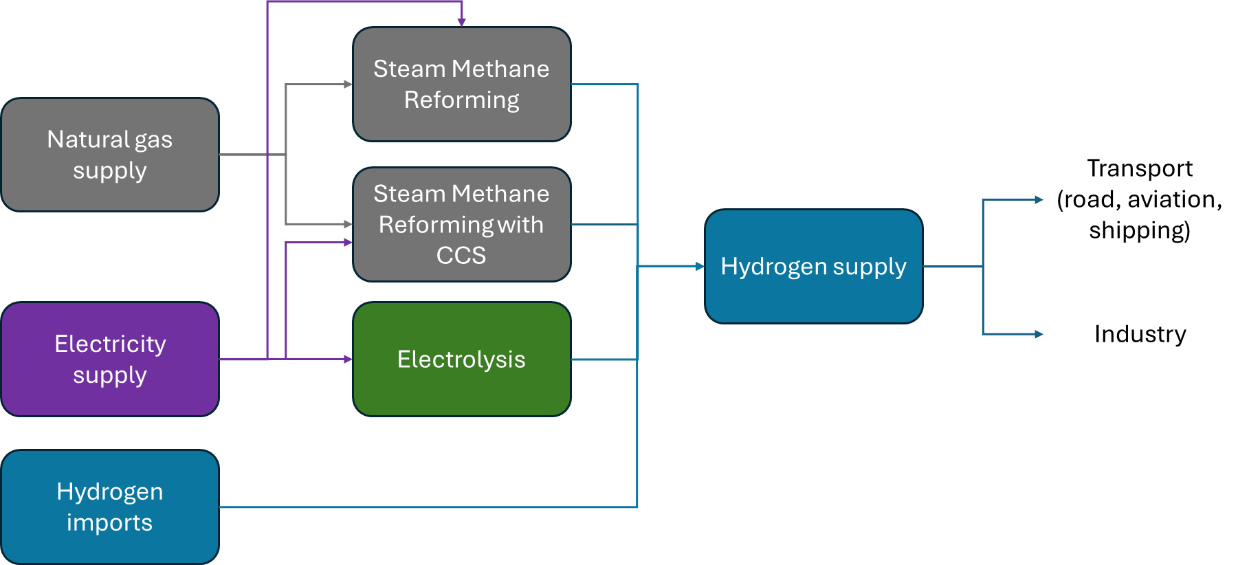
Hydrogen is a fuel whose role may be critical to the decarbonisation of certain sectors. As such, the supply and production of this fuel have to be represented in the CLEWs-EU model. This fuel enters the energy module of the CLEWs-EU model either through imports or domestic production. Production of hydrogen can occur through steam methane reforming (SMR with or without Carbon Capture and Storage) using natural gas as feedstock, or through electrolysis. Hydrogen can then be used in the transport sector or in industry. For use in the aviation sector, hydrogen is first converted into jet fuel.
The technoeconomic assumptions for the relevant hydrogen production technologies are drawn from EU Reference Scenario 2020 assumptions (European Commission - Directorate General for Energy. et al., 2021). Specifically, the adopted input is shown in Table 16.
Technology |
Capital cost (EUR2018/kW) |
Fixed O&M cost (EUR2018/kW) |
Efficiency (energy output vs input) |
||||||
|---|---|---|---|---|---|---|---|---|---|
2021 |
2030 |
2050 |
2021 |
2030 |
2050 |
2021 |
2030 |
2050 |
|
Electrolysis |
1241 |
621 |
186 |
27.5 |
14.5 |
9.3 |
72% |
79% |
85% |
SMR |
564 |
518 |
466 |
22.6 |
20.7 |
18.6 |
70% |
72% |
73% |
SMR with CCS |
927 |
880 |
829 |
37.1 |
35.2 |
33.1 |
41% |
42% |
42% |