Land & Water Module
The land use and water modules are effectively interlinked. Although we use different naming conventions and technologies to represent the two modules in CLEWs-EU, their inputs and outputs are interdependent. The water module represents the following primary sources: water from precipitation and snowmelt (represented as a single entity); water from existing surface and groundwater sources; water from neighbouring geographies through transboundary river exchanges; and water from desalination and secondary sources, such as treatment plants in some countries. The model includes a simplified representation of the water balance for each country. In the land module, the total land available in the continent (in the aggregated model) and in each country (in the disaggregated model) is divided into eight major land categories based on the European Space Agency’s land cover classifications (Eurostat, 2025). These are: grassland, cropland, barren land (including snow-covered areas), water bodies, shrubland, forest cover, built-up land, and wetlands (including mangroves, lichens, and other types of wetlands). Representing land and water systems in a generic systems optimisation setup involves using relevant assumptions to simplify their characterisation while ensuring that little essential detail is lost. Effectively, the land and water modules represent the balance of the two resources (i.e., land and water) in the respective systems. Despite accounting for the balance of these resources, some components, like groundwater storage, are not considered in these modules as they involve detailed subsurface flow modelling, which is outside the scope of the model. Additionally, detailed hydrological water routing across the countries is outside the scope of this work. In the following sections, the overarching assumptions and the technology representation in the land and water module are presented.
Overarching assumptions
In the land and water module, the central assumptions concern the simplifications used to represent the actual setup in each country. In each of the following sections, the country-specific assumptions used in the model are detailed. One common assumption that holds across countries is the growth rate of crop production, which is used as a demand driver in this model. These growth rates (presented in Table 19) are obtained from the European Union’s agricultural outlook 2024-2035 (DG Agriculture and Rural Development, 2024). For crops without a specific growth rate in the outlook, we use an average of all crops, which is also applied to the other (OTH) crop category, which aggregates the crops other than the top ten in each country by planted area. We have maintained the same growth rate between 2035 and 2055, as no specific projections were available for that period.
Crops |
Code |
Average annual growth rate (2024–2035) |
|---|---|---|
Wheat |
WHE |
-0.10% |
Barley |
BRL |
0.10% |
Rape seed |
RAP |
-0.40% |
Rye |
RYE |
0.20% |
Maize |
MAI |
0.40% |
Sugar beet |
SUG |
-0.70% |
Potatoes |
POT |
-0.80% |
Oats |
OAT |
0.20% |
Grapes |
GRP |
-0.80% |
Olives |
OLI |
-0.40% |
Other crops |
OTH |
-0.23% |
Module structure and technological representation
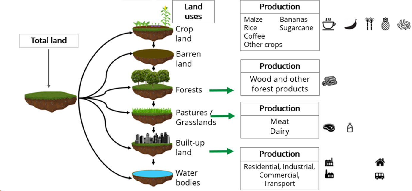
Figure 12 provides a schematic representation of the land component within the broader CLEWs systems framework. The diagram decomposes Total land into distinct land-use categories and their associated products or services. It serves as an illustrative example of how land cover and land use are typically represented in CLEWs models.
Land uses The land module classifies land into several categories, including cropland, barren land, forests, pastures/grasslands, built-up land, water bodies, and wetlands. Each category is linked to a specific type of production activity or ecosystem service.
Production Each land-use category contributes to different outputs:
Cropland supports agricultural production, including crops such as maize, rice, coffee, sugarcane, and others, depending on national cultivation patterns. Crop residues form a portion of the biomass available to the energy system.
Forests provide woody biomass.
Pastures and grasslands support livestock activities, contributing to meat and dairy production.
Built-up land relates to residential, industrial, commercial, and transport services.
The arrows shown in the diagram indicate the flow from land-use categories to their respective outputs. Overall, the illustration highlights the interconnectedness of land systems with food, energy, water, and ecosystem services. It reflects the integrated nature of CLEWs modelling, where changes in land-use policy or resource availability propagate across multiple sectors.
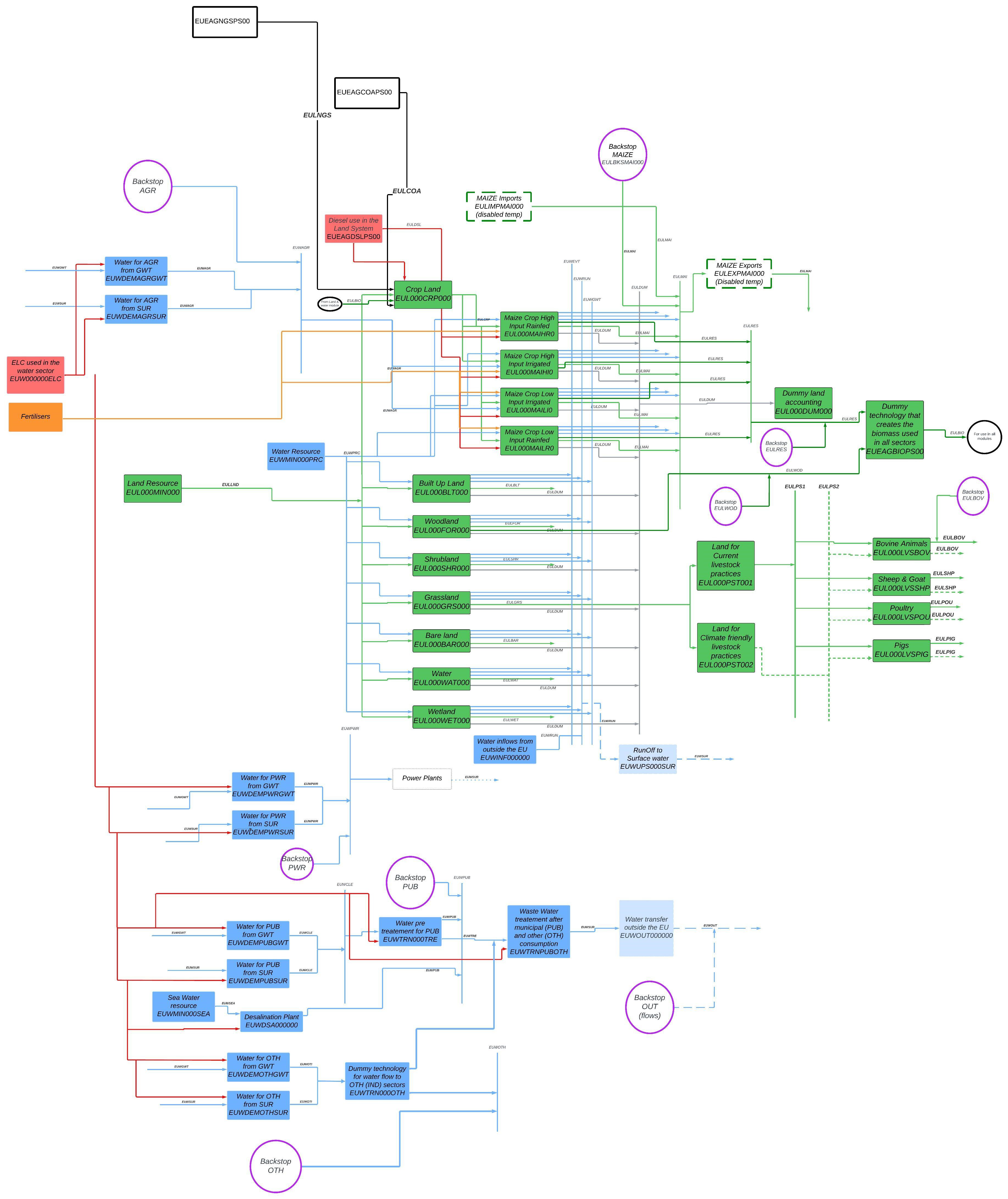
A more detailed system representation is shown in Figure 13, illustrating how the CLEWs-EU land and water modules are formulated, along with their key interactions with the energy module. Solid arrows indicate active links, while dotted arrows denote potential connections that exist in the full CLEWs formulation but are currently disabled to reduce computational load during optimisation.
The diagram is organised by colour, with each group representing a different component of the CLEWs framework:
Land Use (green): This group includes agricultural land (disaggregated into up to ten crop types), barren land, forests, built-up land, water bodies, and wetlands. Each land category is associated with specific outputs—for example, individual crops or contributions to water availability (runoff, infiltration, etc.).
Precipitation and Sea Water (blue): This part of the diagram shows the sources and allocation of water, distinguishing between precipitation-derived surface water, groundwater, and seawater. It highlights the water flows used in agriculture, power generation (PWR), and other sectoral demands.
Energy Supply and Use (red and black): These elements represent the interactions between the energy system and the land and water components, particularly energy use in agriculture and forestry operations, as well as pumping and water treatment processes within the water module.
Interlinkages (arrows of different colours): The arrows illustrate resource flows between the land, water, and energy systems. Examples include water supplied to cropland for irrigation and runoff contributions from each land-use category to surface and groundwater resources.
Backstop technologies (pink): The pink nodes represent modelling constructs included to detect infeasibilities and resource shortages within the optimisation framework.
Fertiliser inputs (orange): This group shows fertiliser applications that enhance crop yields. Some fertilisers used in the model are imported from outside the EU27.
Modelling crop selection and demands
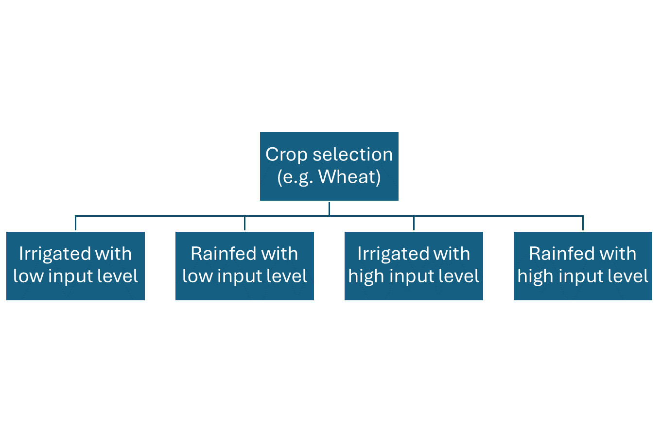
As described earlier, within the cropland category for each country, we rank crops by cultivated area in 2018 and select the top 9, which are represented individually. The remaining crops are grouped together and included in a bundled category. Therefore, there are effectively 10 crop categories, with 9 unique ones represented in each country. The number of crops is lower for countries like Malta and Luxembourg, owing to the total number of crops grown. In the majority of EU27 countries, the top nine crops account for more than 85% of cultivated cropland (FAO, 2024). The crops selected for each country can be accessed in the country-specific input files for the land and water module (on GitHub). For each of these selected crops, two input levels and two water supply options are considered. The input levels (high and low) refer to the degree of mechanisation and the use of fertilisers in the farming techniques, both of which directly influence yield. The water supply options refer to whether the crop is irrigated or rainfed. The water requirement for irrigation is derived from GAEZ’s crop water deficit, which is specific to each crop and the climatic pattern and the country (Fischer, 2021). The different input and water supply combinations available for each crop are presented in Figure 14. As the exact area under irrigation per crop per country is not available, we use the EU-wide average percentage of irrigated area for each crop. We decided to use this value to simplify the representation of irrigation inside the model. For example, crops such as olives have a higher irrigation share (19% of total cultivated area), while crops such as wheat may have a lower share (~2–3%). Overall, the share of cultivated land under irrigation is approximately 7% (Eurostat, 2019).
The EU agricultural outlook (European Commission, 2025) provides projections for major EU agricultural markets until 2035. In this model, the actual production numbers are presented as crop demands until 2023. From 2024, the crop production projections from the outlook have been used to estimate demand for each crop in each EU member state. These growth rates and the assumptions are presented in Table 17. It must be noted that the import and export of crop commodities have not been included in this model. Owing to the uncertainty in price projections and to avoid computational complexity, it has been decided to represent only local production. Having said that, the model provides for the inclusion of exports and imports of any commodity.
Modelling other land categories
The model also considers other landcover types, namely: forests, grasslands (includes pasture), wetlands, built-up lands, barren land, water bodies and shrublands. In this model, the focus is on croplands, forests and grasslands. Therefore, as a common practice in similar modelling studies, we keep the shares of other categories, except built-
Built up land To represent urban growth on artificially built-up land, we use the OECD’s land cover change dataset between 2000 and 2020 and use the 20-year CAGR for each country (Vladimir Tesnière, Mikaël J. A. Maes, Ivan Haščič, 2024). This process involves using the raw GIS data to compute the final numbers. The country-specific values are available on the public GitHub repository.
Forests and grasslands expansion The area in forests and grasslands is given an economic incentive to maintain land under their cover. It is also essential to highlight that they have GHG sequestration potential, which varies by country. The incentive presented as negative variable costs is basically a way to represent the opportunity cost of removing the forests and grasslands for agriculture and other purposes. We have maintained these costs unchanged across all countries, as it was not possible to estimate an opportunity cost for each country. This is also one of the limitations of the model, as highlighted in section 2.2. Additionally, the forests and grasslands in each country have maximum growth rates aligned with national policies. These values are derived from national projections. The maximum annual growth rate is limited from 2024 onward, as actual land cover values are only available through 2023.
Energy use in the land and water module
Energy used in the water and land use module is modelled by linking the energy inputs (fossil fuels and electricity) from the energy module with the respective end-use sectors. Electricity is used in the agricultural sector for pumping water from surface and groundwater sources, for treating water before sending it for consumption in households, and for treating water after use to be let out into surface water bodies. Figure 15 presents the section of the system where the electricity flows from the energy module are provided as inputs to the pumping technologies that supply water for irrigation, cooling in thermal power plants and supply to other commercial and industrial needs. The energy use factors for pumping were obtained from (Plappally & Lienhard V, 2012). The efficiencies and the cost of both types of treatment mentioned above are obtained from ((Paraschiv et al., 2023; Schiller & Dirlich, 2015; Urban Waste Water Directive Treatment Plants Data Viewer, 2017). We assume a uniform energy intensity for all the countries. The cost of treatment always includes an energy component. We have attempted to remove this component to prevent double-counting. However, this section could be improved with more actual project-specific costs. Additionally, the national-level energy balances (Rózsai et al., 2024) have been used to account for all other energy flows to the agriculture and forestry sectors. To simplify the representation of these energy inputs, we subtracted the total energy for pumping and diesel consumption in the land-use sector from the total energy used (by fuel) in the Agricultural and forestry sector. This resulting value was divided by the total cropland area to derive the energy intensity per unit area of cultivated cropland in each EU-27 country. These fuels were disaggregated into Diesel, Natural Gas, Coal and biomass fuel (which includes biomass, biofuel and other bio-based energy commodities found in the energy balance). We used these intensities to calibrate energy consumption in the agriculture and land-use sector.
Water use and consumption
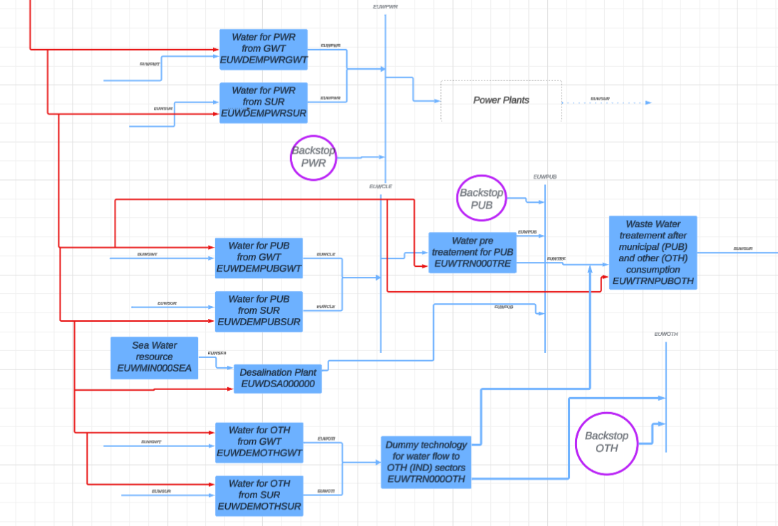
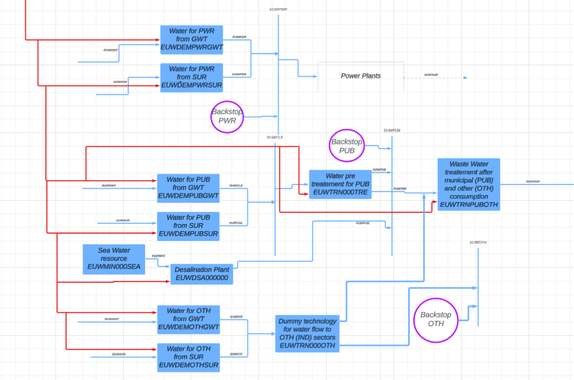
In the CLEWs-EU model, the demands for water in the power, agriculture, and domestic use sectors are modelled explicitly. All other water use, predominantly the commercial and industrial sectors, is grouped into the “Other” category. Water used for cooling thermal power plants and for irrigation of cropland is endogenously determined within the model. Figure 16 highlights the structure of the water supply to the respective end uses. For household use, the water is first treated before supply, and the wastewater is channelled through a technology that represents post-use treatment before being returned to surface water sources.
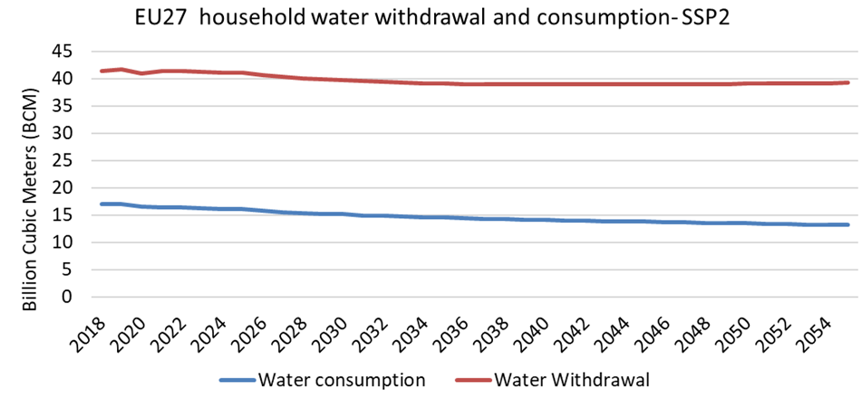
Water use in the residential sector The demand (withdrawal and consumption) for water in the residential sector was obtained from (Fridman et al., 2024). These values are calibrated against actual numbers from Eurostat. The data set has different projections available until 2100. We assume a median projection from SSP2 for the base scenario. Figure 17 presents the values for all the EU27 countries together. The values are expected to decline owing to an expected decline in the population and lower per capita water use.
Water use in the commercial and industrial sectors
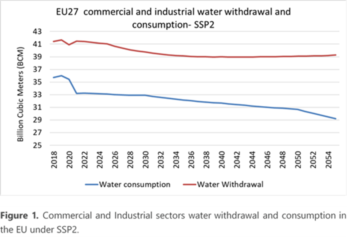
The demand (withdrawal and consumption) for water in the commercial and industrial sectors was obtained from (Fridman et al., 2024). These values are calibrated against actual numbers from Eurostat. The data set has different projections available until 2100. We assume a median projection from SSP2 for the base scenario. Figure 18 presents the values for all the EU27 countries together. The values are expected to decline due to a projected decrease in population and lower per capita water use. Like the household projections, the demand for water in these sectors is also expected to decline.
Water use in the power sector
Thermal power plants (fossil fuel, biomass, Nuclear, etc.) need to be cooled, and water is used in most of them. There are two primary types of water-based cooling technologies: once-through cooling (direct) and wet-recirculating/closed-loop (indirect). Sometimes the water used for cooling is from a nearby river, pond, or even seawater. In our model, we simplify the representation of water for cooling in thermal power plants. We calibrate the water used for cooling (obtained as a single number per country and year) from Eurostat with the total electricity generation from thermal power plants to calculate a cooling water withdrawal and consumption intensity, presented per unit of electricity produced. This methodology provides us with good accuracy in water withdrawal and consumption, eliminating the need to represent cooling technologies and thereby reducing the computational load. Table 20 presents the water withdrawal for cooling in thermal power plants in the EU27 countries. The data was obtained for Eurostat
Country |
Thermal electricity generation (PJ) |
Water withdrawal (MCM) |
|---|---|---|
Austria |
291.61 |
1495.1 |
Belgium |
142.44 |
2256.5 |
Bulgaria |
20.45 |
3471.7 |
Croatia |
15.86 |
167.3 |
Cyprus |
282.27 |
14.8 |
Czechia |
56.42 |
264.5 |
Denmark |
21.94 |
3.5 |
Estonia |
170.17 |
681.7 |
Finland |
1575.11 |
405.4 |
France |
1444.75 |
14368.4 |
Germany |
118.87 |
13321.6 |
Greece |
112.65 |
Data not available |
Hungary |
75.49 |
3586.7 |
Ireland |
680.88 |
359.2 |
Italy |
10.76 |
4594.2 |
Latvia |
8.06 |
2.6 |
Lithuania |
2.27 |
87.5 |
Luxembourg |
7.05 |
Data not available |
Malta |
331.68 |
Data not available |
Netherlands |
562.60 |
3183.3 |
Poland |
78.82 |
5216 |
Portugal |
120.41 |
786.9 |
Romania |
89.02 |
566 |
Slovakia |
37.52 |
50.4 |
Slovenia |
291.61 |
717.1 |
Spain |
547.23 |
4682.7 |
Sweden |
248.77 |
113.4 |
Livestock representation
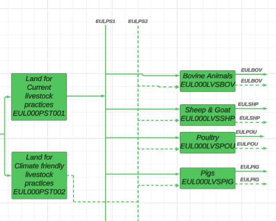
In the CLEWs-EU model, the land used for livestock farming and the corresponding GHG emissions are modelled. The livestock representation includes bovine animals (cattle, etc.), pigs, sheep, goats, and poultry (Figure 19). The demands for livestock are exogenously defined in the model. In the model, livestock demand is defined as a function of the live head count for each animal category. Additionally, the demand is specified in Livestock Units (LSU) rather than individual animal categories. The assumptions for the conversions were derived from a European Commission study on livestock greenhouse gas emissions (Leip & Weiss, 2010). The assumptions for the land footprint of the livestock are obtained again from a modelling study conducted by the European Commission (De et al., 2022). The figure below provides a simplified representation of the livestock sector. We have made provisions in the model to develop an analysis that takes into consideration more climate-friendly agricultural practices. The main objective of representing livestock is to capture the GHG emissions and account for the land used to maintain them.
Biomass production
Biomass (woody biomass, crop residue, biofuels, biodegradable waste and other bio-derived sources of energy) is used in all sectors in varying amounts. Approximately 96% of all the biomass used in the EU-27 countries is sourced within its borders. However, this share is different from country to country. For example, Cyprus imports a significant share of its biomass used in various local sectors, whereas the share is lower in Ireland. The National Renewable Energy Action Plans (NREAPs) for each EU-27 country specify the share of woody biomass, agricultural residue and other sources of biomass supply (Scarlat et al., 2019). In this model, to simplify the representation of biomass availability, we have two main categories: woody biomass from forests and all the other sources represented as agricultural residue. The woody biomass energy potential for each member state is calculated using the forested area in each country, the country-wide average wood intensity, the LHV value and the availability factor of wood for energy purposes (Avitabile et al., 2024). These values were calibrated for the base year, and an intensity of woody biomass per unit of forested area was calculated. Table 21 presents the potential for each EU-27 member state.
Country |
Woody biomass energy potential – Intensity (PJ/1000 sqkm/year) |
|---|---|
Austria |
1.68 |
Belgium |
2.125 |
Bulgaria |
1.123 |
Croatia |
1.634 |
Cyprus |
0.333 |
Czechia |
2.308 |
Denmark |
3.169 |
Estonia |
1.527 |
Finland |
1.11 |
France |
1.608 |
Germany |
2.783 |
Greece |
0.867 |
Hungary |
1.587 |
Ireland |
2.588 |
Italy |
0.947 |
Latvia |
1.55 |
Luxembourg |
2.03 |
Malta |
0.333 |
Netherlands |
2.087 |
Poland |
2.125 |
Portugal |
1.40 |
Romania |
1.184 |
Slovakia |
1.847 |
Slovenia |
1.894 |
Spain |
0.68 |
Sweden |
0.897 |
Lithuania |
1.905 |
The component of biomass from agricultural residues is calculated using the Residue-to-Product-Ratio (RPR), the LHV for each crop and the surplus availability factor (SAF). These are calculated for each crop type and used in the model as output activity ratios for each crop-producing technology in each country. The detailed methodology for the calculation is provided in (Singhal et al., 2024) and the associated GitHub repository.
Data sources
The construction of the Land and Water modules within the CLEWs-EU framework necessitates an extensive acquisition and processing of data. Table 22 delineates a summary of the primary data requisites pertinent to the land and water components of the model. In alignment with the approach adopted for the energy module, we are collecting data at the individual country level, despite the initial development focus on a regional EU aggregate. For land, this includes data on land use patterns, agricultural productivity, and forest cover policies, among others. For water, we gather information on water availability, usage statistics across sectors, withdrawal limits, and water use intensities. Exceptions are made for general hydrological parameters and land management practices, where universally applicable figures are employed in the preliminary stages. Nevertheless, country-specific calibration is still essential to enhance accuracy and relevance, particularly in reflecting the unique hydrological and agricultural conditions of each member state.
Sector |
Data item |
Primary Source |
|---|---|---|
Land Cover |
Area under different land cover classes Area under crop cultivation Emission factors |
FAO, Eurostat, European Space Agency (WorldCover2021) Aquastat & Eurostat Eurostat and European GHG Inventory |
Agriculture |
Crop yields and production statistics Fertiliser usage in crop production Crop import statistics Costs involved in crop production Fuel usage in agriculture and forestry |
Global Agro-Ecological Zoning (GAEZ – FAO/IIASA), Magpie modelling group Eurostat, peer-reviewed literature FAOSTAT National statistics, Eurostat, derived values JRC IDEES – Energy Balances |
Water Availability and Use |
Precipitation statistics Groundwater potential Water use factors in different sectors Evapotranspiration under different land categories Demand projections for water in different sectors |
Eurostat, GAEZ Peer-reviewed journals, Eurostat Eurostat GAEZ IIASA projections calibrated with Eurostat |